Guide to Antenna Matching

Using nanoVNA, QucsStudio, and MatchCalc.

Disclaimer: I am not an RF engineer, and the methods described here may not be ideal or "right," but they have worked for me.

Recently, I was tasked with designing a BLE device with a ceramic chip antenna. As expected, the antenna needed to be matched, since the matching element designed by its manufacturer could not be used due to differences in the PCB stackup.

After researching and experimenting, I developed a relatively easy and fast method that enabled me to tune the antenna with only three measurement and adjustment cycles.

Step 1: Measure Parameters with nanoVNA

Assuming you have no experience with this, let's go over some basics of nanoVNA measurement.
We will focus only on single-port measurements.

Calibration Plane

Calibrating your VNA is crucial for obtaining useful measurements.
In my case, I performed the calibration of the VNA with a coaxial cable attached directly to the PCB feed line. Since the PCB was designed to be populated with a matching network, I could perform all open, short, and load calibration steps without removing the coax from the PCB.

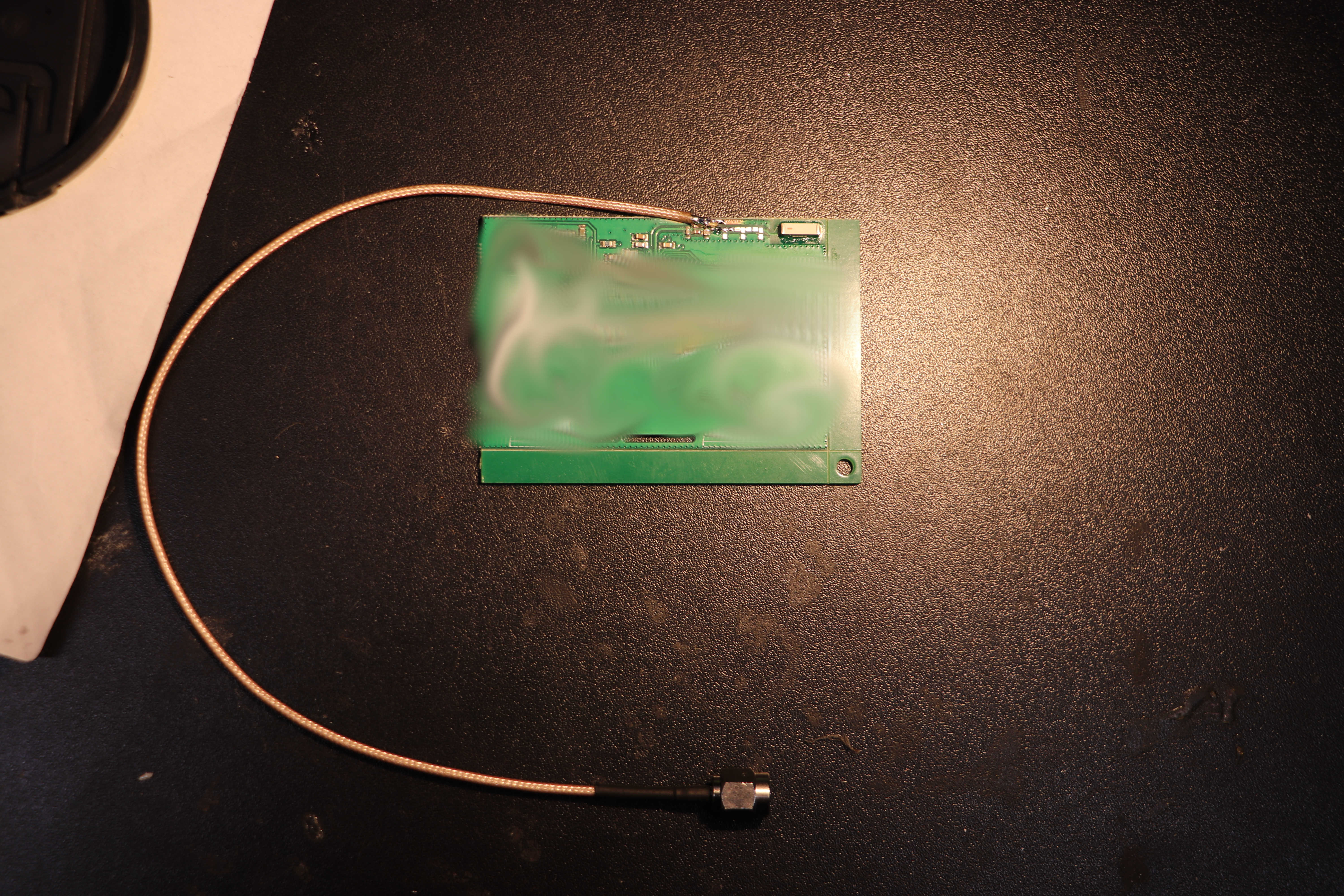
In the pictures above, you can see a piece of RG178 coaxial cable with an SMA connector connected to the PCB.
The end of the coax has its shield soldered to the PCB's ground plane, which was stripped of its resist, with its inner conductor soldered to an SMD pad.
During the process, we cannot move this in order to not change our calibration plane.

Calibrating nanoVNA

In nanoVNASaver, we set the desired frequency range and number of segments.

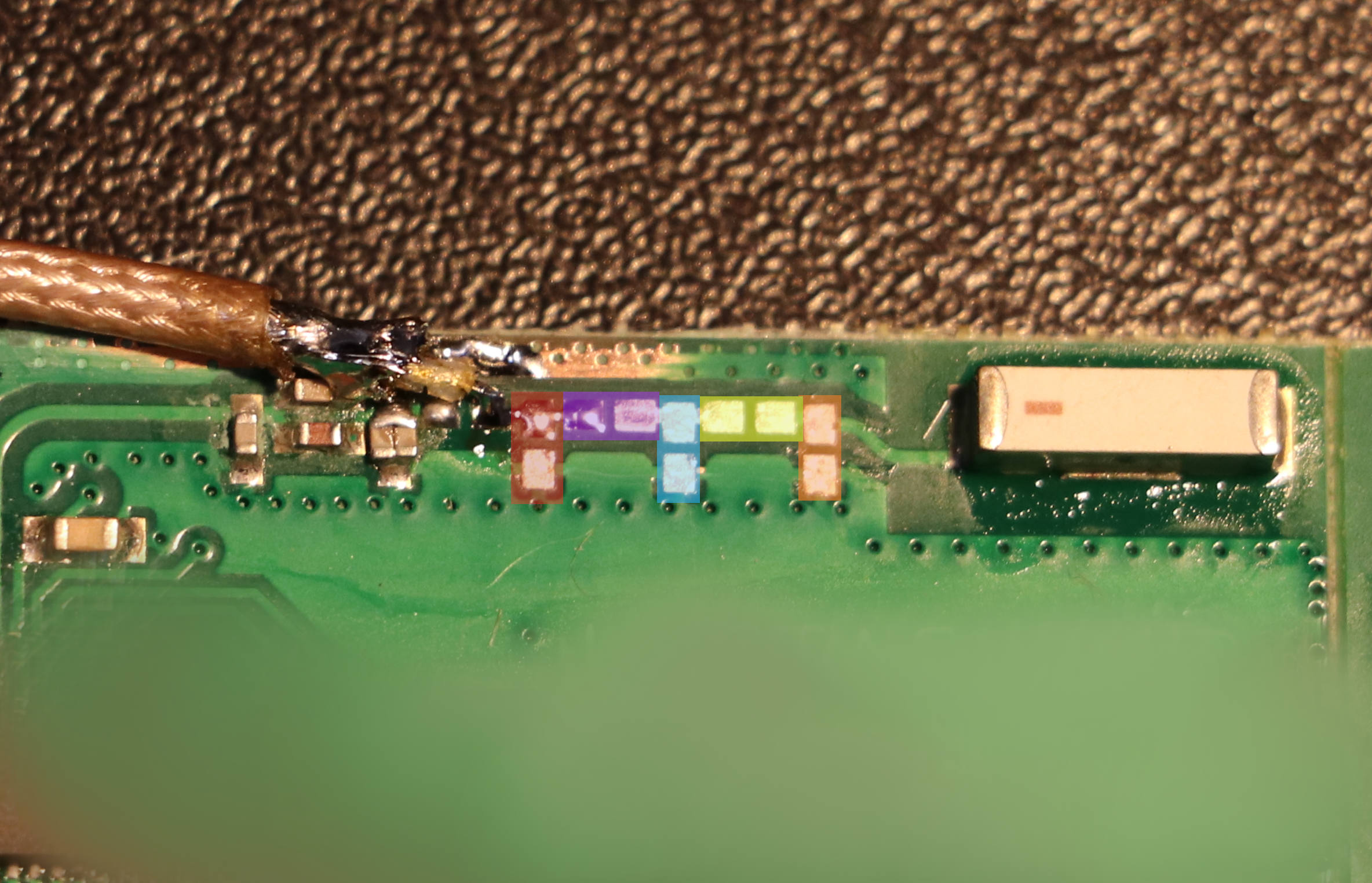
Now we perform the nanoVNA calibration using the nanoVNASaver calibration helper. We'll be asked to connect a short standard, which we create by shorting pads highlighted in red. Then the open standard, created by removing the previously created short. Lastly, the load standard, created by soldering a 50Ω resistor to pads highlighted in red.

After this, we have successfully calibrated the VNA and we'll proceed with the antenna measurement.

First Antenna Measurement

Connect the antenna to the coax by populating 0Ω resistors (or just with solder jumpers) on the purple and yellow pads.
In nanoVNASaver, start the sweep by clicking the Sweep button. This measurement can take a few minutes, during which we shouldn't touch or manipulate the DUT (Device Under Test).

After the measurement is finished, save the measured single port data: Files -> Export single port file (S1P).

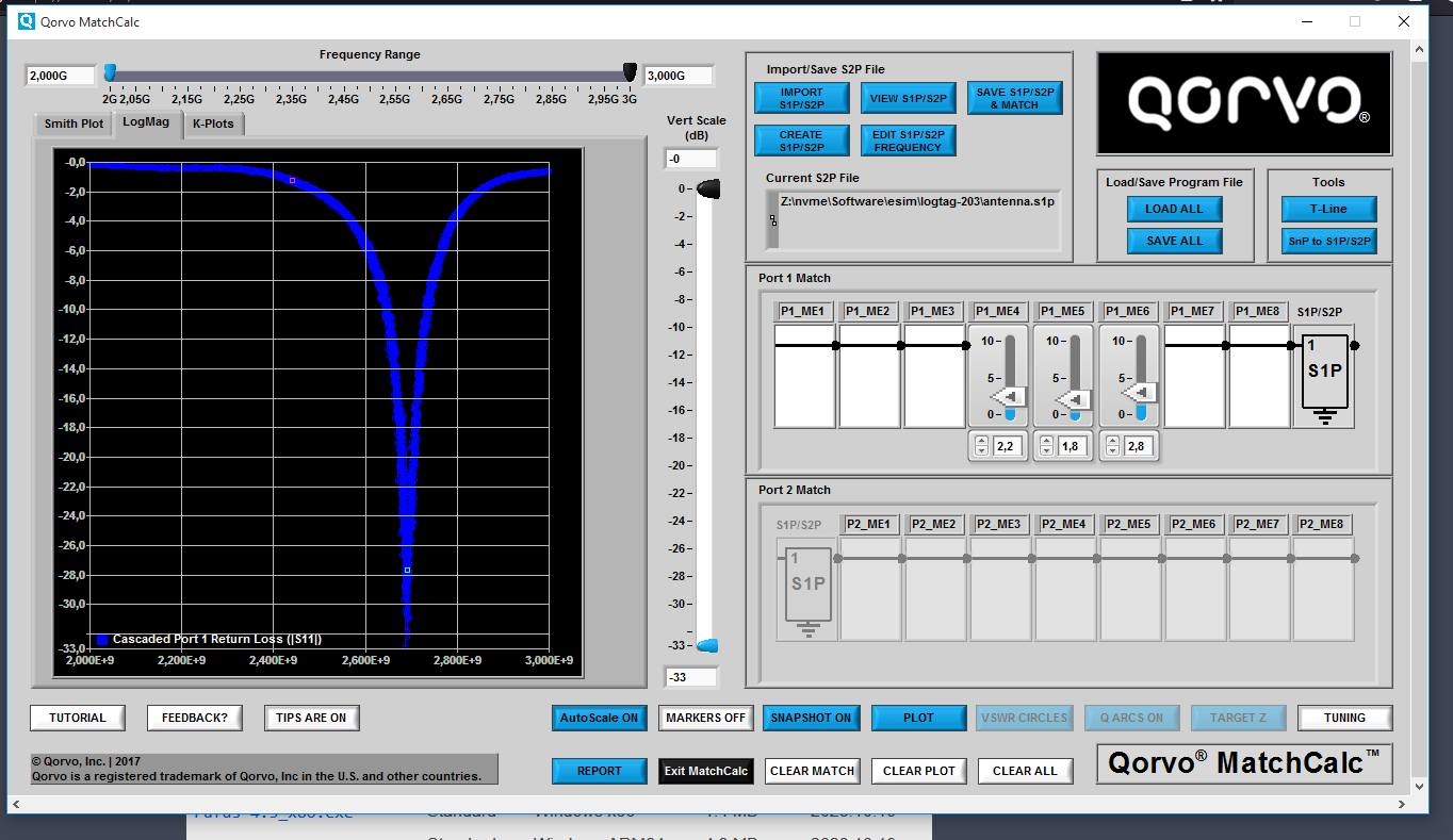
Step 2: Find Crude Matching Network Component Values

For finding initial values of matching network components, I found a useful tool, MatchCalc™ by Qorvo.
Unfortunately, it's a Windows-only program and I couldn't manage to get it running under Wine, so I used a VM.
I suggest starting with this short tutorial, but the tool itself is super easy to use, so you can probably skip it.

In MatchCalc, we start by loading data from nanoVNASaver and selecting plots Cascaded Port 1 Return Loss and Cascaded Port 1 Impedance.
Optionally, we can add a marker for our target frequency for better tracking.

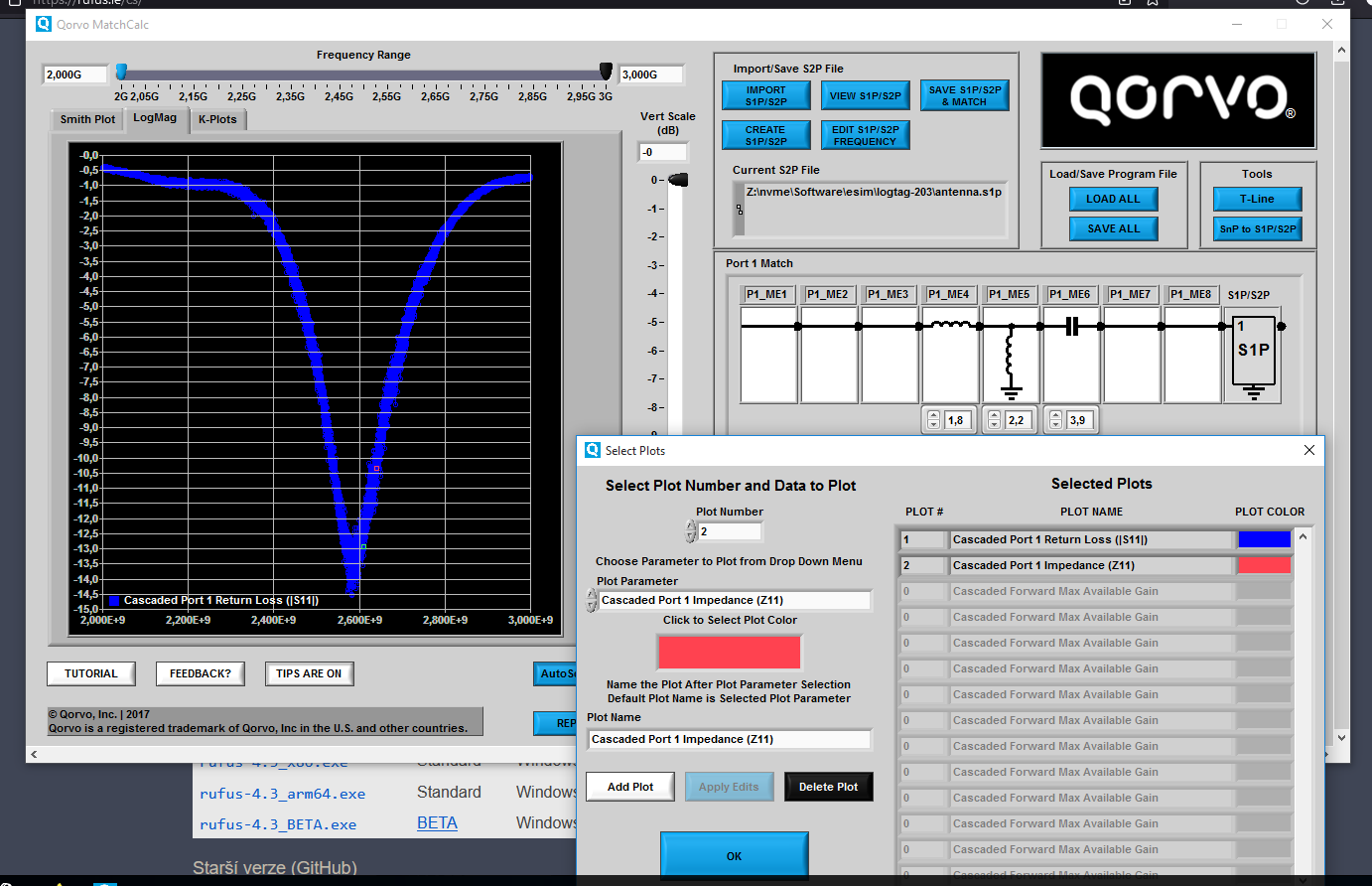
After that, add various components in the Port 1 Match section. By clicking the TUNE button, we can enable sliders for adjusting the values of chosen components.

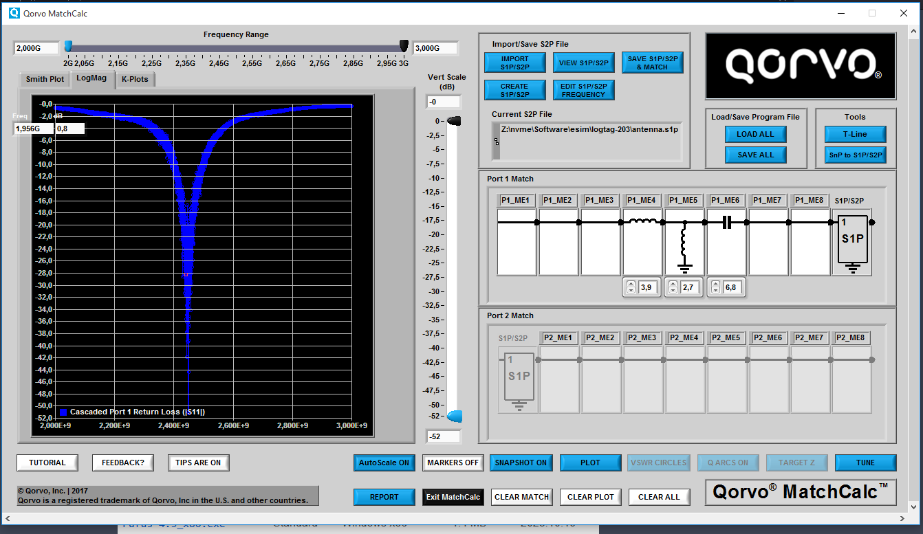
For my first try, I landed on values of a series 3.9nH, a shunt 2.7nH, and a series 6.8pF.

Step 3: Verify Chosen Matching Components with QucsStudio

QucsStudio is a Windows-only program, but it runs under Wine just fine.

Now, we verify if the simulation in QucsStudio yields the same results as in MatchCalc. This step might be skipped, but I've done it because MatchCalc is only a general-purpose simulator.

To perform a simulation with QucsStudio, you can use this schematic file. You'll need to modify paths to S1P files as well as parameters of the simulation.

Then, run the simulation by pressing F2 and see if the results are the same as in MatchCalc.

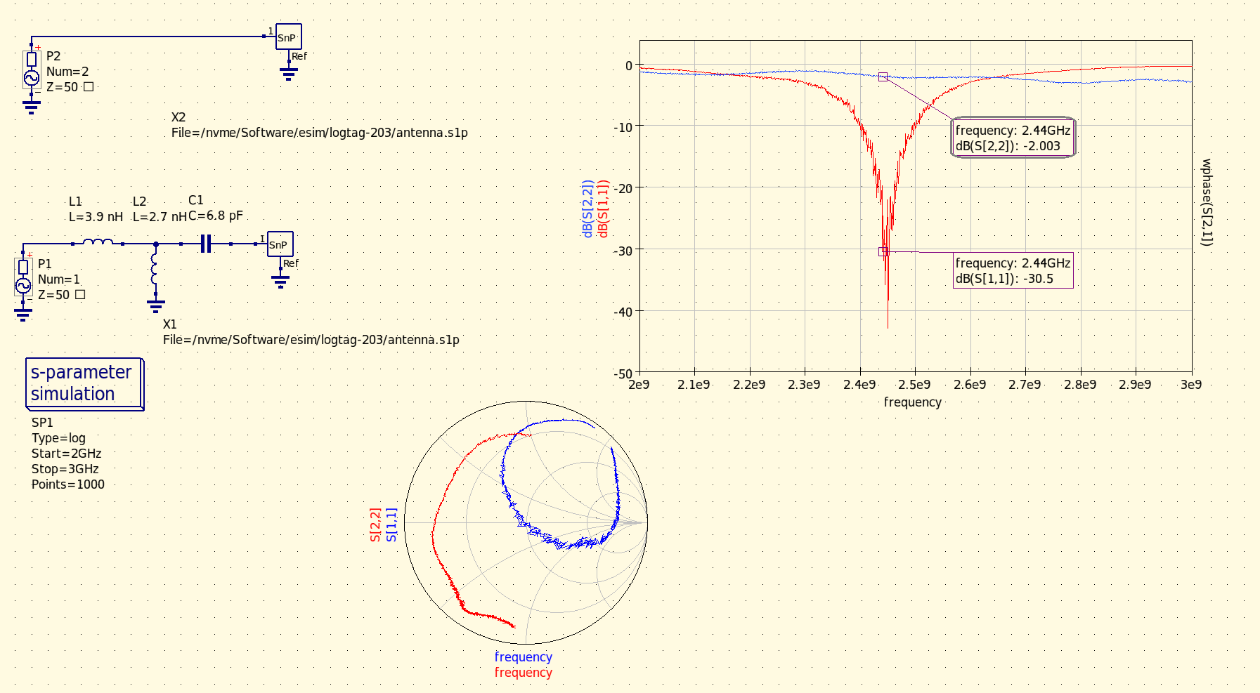
Then populate our matching element with components from the simulation.

Step 4: Matched Antenna Measurement

Now we should have an antenna with a matching element. Repeat the steps from the section First Antenna Measurement and save the data.

Continue with loading our file to QucsStudio as X2. Press F2 to run the simulation to plot graphs for the new measurement.

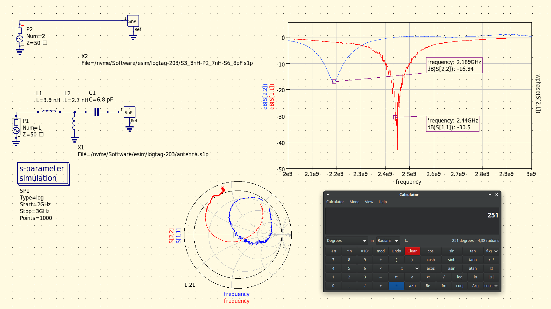
We can see that the matching element part values from the first simulation resulted in the antenna being tuned to a lower frequency than the target.

Use graph markers to get the frequency of the lowest S11 value and calculate the difference between the current and target frequency.

We can see that our antenna is tuned ~251MHz lower.

Now we return back to MatchCalc, where we place a new marker on the frequency (2.44+0.251) 2.691GHz.
Then tune the component values again to achieve the best match on the newly marked frequency.

Then we change components on the DUT and repeat the measurement with the VNA and check the results.

Step 5: Finalization

I found out that you can fine-tune the matching network even with results from simulations that are deviating from real-world results by using simulation in relative mode.
For example, if you know that your antenna is tuned 100MHz lower, you can tweak component parameters and find that decreasing capacitance by 1pF tunes it the desired 100MHz higher.
Then, you simply adjust your current values based on what you simulated.
This way, I was able to match my antenna in just four measurement and tuning cycles.

Software

Initially, I tried to simulate this in Qucs-S, but it turned out that all available solvers are not able to simulate single-port devices.
The only option for that is QucsStudio, thankfully it's free.
It should be possible to run MatchCalc™ under Wine, but I struggled with the correct versions of of Visual C++ and .NET.